dat_2015 <- read.csv("https://raw.githubusercontent.com/elisefeld/elise_data_dump/main/Combined_2015_data.csv") |>
  clean_names() |>
  mutate(across(everything(),
                str_remove_all,
                pattern = fixed(" "))) |> #remove spaces in data
  mutate(across(where(is.character),
                ~na_if(., "null"))) |> #add null vals for chrs
  mutate(across(c(tree_number,
                  subplot),
                as.character)) |> #convert to chr datatype
  mutate(across(c(plot_year,
                  plot_month,
                  height,
                  dbh),
                as.numeric)) |> #convert to numeric datatype
  rename(dbh_2015 = dbh,
          note_2015 = note,
plot_month_2015 = plot_month) EREN Research Project Analysis
ggplot
BIO 261: Ecological Principles
Statistical Analysis and Visualization for EREN Plot Data
This analysis comapres EREN plot data collected by BIO 261’s lab groups in 2024 to historical data from 2015, focusing on the growth and health of tree species within various ecological plots. The dataset includes measurements from 2015 and 2024, allowing us to examine changes over nearly a decade. The analysis includes data cleaning, data transformations, statistical tests, and visualizations to explore relationships between tree characteristics and plot conditions.
Data Preparation and Cleaning
We start by importing and cleaning the datasets from 2015 and 2024 by removing spaces, handling null values, and standardizing data formats.
Cleaning 2015 Data
Cleaning 2024 Data
dat_2024 <- read.csv("https://raw.githubusercontent.com/elisefeld/elise_data_dump/main/Combined_2024_data.csv") |>
  clean_names () |>
  select(-group) |>
  mutate(across(everything(),
                str_remove_all,
                pattern = fixed(" "))) |> #remove spaces in data
  mutate(across(where(is.character),
                ~if_else(. %in% c("",
                                  "unidentified",
                                  "Dead/Missing",
                                  "null",
                                  "na",
                                  "NA",
                                  "Na"),
                          NA_character_, .))) |> #add null vals for chrs
  mutate(plot_month = str_replace(plot_month, "September", "9"),
         plot_name = str_replace_all(plot_name, c("_" = "",
                                                  "Plot4" = "southsouth",
                                                  "4" = "southsouth",
                                                  "northeast" = "northnorth",
                                                  "notheast" = "northnorth")),
         plot_name = str_to_lower(plot_name)) |> #standardizes plot_name & plot_month cols
   mutate(across(c(height,
                   dbh),
                 na_if, "0")) |> #add null vals for nums
   mutate(dbh = na_if(dbh, "61.5")) |> #REMOVING OUTLIER DBH
   mutate(across(c(height,
                   dbh,
                   plot_year,
                   plot_month),
                 as.numeric)) |> #convert to numeric datatype
   mutate(across(c(height,
                   dbh),
                 round, 2)) |> #round values to 2 decimal places
   rename(dbh_2024 = dbh,
          note_2024 = note,
          height_2024 = height,
          plot_month_2024 = plot_month)
Preparation and Joining
The cleaned datasets are further processed to combine duplicated measurements for each tree, calculate growth rates, and identify dead trees. This allows for easy comparison of changes between 2015 and 2024.
#averaging trees that were measured more than once in each data set
dat_2015_new <- dat_2015 |>
    group_by(plot_name,
             tree_number) |>
    mutate(plot_month_2015 = Mode(plot_month_2015),
           dbh_2015 = mean(dbh_2015,
                           na.rm = TRUE)) |> #taking the mean dbh of all trees with the same plot name and tree number
  distinct(tree_number,
           .keep_all = TRUE) |>
  select(-plot_year,
         -plot_month_2015)


dat_2024_new <- dat_2024 |>
  group_by(plot_name,
           tree_number) |>
  mutate(plot_month_2024 = Mode(plot_month_2024),
         dbh_2024 = mean(dbh_2024,
                         na.rm = TRUE),
         height_2024 = mean(height_2024,
                            na.rm = TRUE)) |> #taking the mean dbh and height of all trees with the same plot name and tree number
  distinct(tree_number,
           .keep_all = TRUE) |>
  mutate(across(where(is.numeric),
                ~na_if(., NaN))) |> #changing not a number to NA
  select(-plot_year,
         -plot_month_2024)
Joining & Creating New Variables
dat_all <- dat_2024_new |>
    left_join(dat_2015_new,
              by = c("plot_name",
                     "subplot",
                     "tree_number")) |>
    select(plot_name,
           subplot,
           tree_number,
           species_code.y,
           dbh_2015,
           dbh_2024,
           height_2024,
           note_2015,
           note_2024,
           inv_status,
           stemtype,
           soundness,
           crownclass,
           treedamage) |>
  rename(species_code = species_code.y) |>
  mutate(treedamage = str_to_upper(treedamage),
         growth_factor = (dbh_2024 - dbh_2015) / 9, #create growth factor col, 2024-2015/9yrs
         dead_2015 = note_2015, #copy col
         dead_2024 = note_2024) |> #copy col
  mutate(dead_2015 = case_when(str_detect(dead_2015, "lvsgone") ~ "DEADNOLEAVES",
                               str_detect(dead_2015, "noleavesleft")  ~ "DEADNOLEAVES",
                               str_detect(dead_2015, "leavesgone")  ~ "DEADNOLEAVES",
                               str_detect(dead_2015, "fewleaves")  ~ "DEADNOLEAVES",
                               str_detect(dead_2015, "leavesallgone")  ~ "DEADNOLEAVES",
                               str_detect(dead_2015, "mostleavesgone")  ~ "DEADNOLEAVES",
                               str_detect(dead_2015, "dead") ~ "DEAD",
                               TRUE ~ dead_2015)) |> #if contains left, convert to right
  mutate(dead_2015 = replace(dead_2015,
                             !grepl("DEAD", dead_2015),
                             "NODATA")) |>
  mutate(dead_2024 = case_when(str_detect(dead_2024, "noleaves") ~ "DEADNOLEAVES",
                               str_detect(dead_2024, "dead") ~ "DEAD",
                               str_detect(dead_2024, "missing") ~ "DEAD",
                               str_detect(dead_2024, "Gone") ~ "DEAD",
                               str_detect(dead_2024, "Dead") ~ "DEAD",
                               str_detect(dead_2024, "deceased") ~ "DEAD",
                               TRUE ~ dead_2024)) |> #if !contain DEAD, convert to NODATA
   mutate(dead_2024 = replace(dead_2024,
                              !grepl("DEAD", dead_2024),
                              "NODATA")) |> #if !contain DEAD, convert to NODATA
   mutate(species_name = as.factor(species_code),
          species_genus = as.factor(species_code)) |>
   mutate(species_name = fct_recode(species_name,
                                    "Amur Maple" = "ACEGIN",
                                    "Boxelder" = "ACENEG",
                                    "Red Maple" = "ACERUB",
                                    "Sugar Maple" = "ACESAC",
                                    "Bitternut Hickory" = "CARCOR",
                                    "American Ash" = "FRAAME",
                                    "Black Walnut" = "JUGNIG",
                                    "Eastern Hophornbeam" = "OSTVIR",
                                    "Bigtooth Aspen" = "POPGRA",
                                    "Black Cherry" = "PRUSER",
                                    "Chokecherry" = "PRUVIR",
                                    "White Oak" = "QUEALB",
                                    "Bur Oak" = "QUEMAC",
                                    "Red Oak" = "QUERUB",
                                    "Common Buckthorn" = "RHACAT",
                                    "American Basswood" = "TILAME",
                                    "American Elm" = "ULMAME")) |> #create new col species_name
   mutate(species_genus = fct_collapse(species_genus,
                                       Acer = c("ACEGIN", "ACENEG", "ACERUB", "ACESAC"),
                                       Caryus = c("CARCOR"),
                                       Fraxinus = c("FRAAME"),
                                       Juglans = c("JUGNIG"),
                                       Ostrya = c("OSTVIR"),
                                       Populus = c("POPGRA"),
                                       Prunus = c("PRUSER", "PRUVIR"),
                                       Quercus = c("QUEALB", "QUEMAC", "QUERUB"),
                                       Rhamnus = c("RHACAT"),
                                       Tilia = c("TILAME"),
                                       Ulmus = c("ULMAME"))) |> #create new col species_genus
    mutate(plot_name_num = case_when(str_detect(plot_name, "northnorth") ~ 2,
                                  str_detect(plot_name, "northsouth") ~ 1,
                                  str_detect(plot_name, "southnorth") ~ 3,
                                  str_detect(plot_name, "southsouth") ~ 4,)) |> #plot name chr to numeric
    mutate(hl_density = case_when(str_detect(plot_name, "northnorth") ~ "Low Density",
                                  str_detect(plot_name, "northsouth") ~ "Low Density",
                                  str_detect(plot_name, "southnorth") ~ "High Density",
                                  str_detect(plot_name, "southsouth") ~ "High Density")) |> #new col plots high or low density
    mutate(species_name = as.factor(species_name))
Pivoting for Visualization
dat_all_pivot <- dat_all |>
  pivot_longer(cols = starts_with("dbh_"),
               names_to = "year",
               values_to = "dbh",
               names_prefix = "dbh_")
#How many of each species are in each plot?
tbl1 <- table(dat_all$species_name, dat_all$plot_name)
tbl1
                      northnorth northsouth southnorth southsouth
  American Ash                 3         43         18         45
  Bur Oak                     24          1          0          0
  Bigtooth Aspen               1          0          0          0
  White Oak                   18          1          0          0
  Red Oak                      2          0          1          0
  Sugar Maple                  8          5          0          2
  American Basswood            4          0          0          0
  American Elm                 5          3          0          0
  Bitternut Hickory            1          0          0          0
  Chokecherry                  1          1          0          0
  Black Cherry                 1          1          0          0
  Black Walnut                 0          3         13          7
  Boxelder                     0          5          4          2
  Eastern Hophornbeam          0          5          0          0
  Common Buckthorn             0          1          0          0
  Red Maple                    0          0         24          5
  Amur Maple                   0          0          6          0
prop1 <- prop.table(tbl1, margin = 1)
prop1
                      northnorth northsouth southnorth southsouth
  American Ash        0.02752294 0.39449541 0.16513761 0.41284404
  Bur Oak             0.96000000 0.04000000 0.00000000 0.00000000
  Bigtooth Aspen      1.00000000 0.00000000 0.00000000 0.00000000
  White Oak           0.94736842 0.05263158 0.00000000 0.00000000
  Red Oak             0.66666667 0.00000000 0.33333333 0.00000000
  Sugar Maple         0.53333333 0.33333333 0.00000000 0.13333333
  American Basswood   1.00000000 0.00000000 0.00000000 0.00000000
  American Elm        0.62500000 0.37500000 0.00000000 0.00000000
  Bitternut Hickory   1.00000000 0.00000000 0.00000000 0.00000000
  Chokecherry         0.50000000 0.50000000 0.00000000 0.00000000
  Black Cherry        0.50000000 0.50000000 0.00000000 0.00000000
  Black Walnut        0.00000000 0.13043478 0.56521739 0.30434783
  Boxelder            0.00000000 0.45454545 0.36363636 0.18181818
  Eastern Hophornbeam 0.00000000 1.00000000 0.00000000 0.00000000
  Common Buckthorn    0.00000000 1.00000000 0.00000000 0.00000000
  Red Maple           0.00000000 0.00000000 0.82758621 0.17241379
  Amur Maple          0.00000000 0.00000000 1.00000000 0.00000000
dat_all |>
tabyl(species_name, plot_name) |>
adorn_totals(c("row", "col")) |>
adorn_percentages(denominator = "col") |>
adorn_pct_formatting() |>
adorn_ns() |>
knitr::kable()| species_name | northnorth | northsouth | southnorth | southsouth | Total |
|---|---|---|---|---|---|
| American Ash | 4.1% (3) | 58.1% (43) | 24.7% (18) | 69.2% (45) | 38.1% (109) |
| Bur Oak | 32.4% (24) | 1.4% (1) | 0.0% (0) | 0.0% (0) | 8.7% (25) |
| Bigtooth Aspen | 1.4% (1) | 0.0% (0) | 0.0% (0) | 0.0% (0) | 0.3% (1) |
| White Oak | 24.3% (18) | 1.4% (1) | 0.0% (0) | 0.0% (0) | 6.6% (19) |
| Red Oak | 2.7% (2) | 0.0% (0) | 1.4% (1) | 0.0% (0) | 1.0% (3) |
| Sugar Maple | 10.8% (8) | 6.8% (5) | 0.0% (0) | 3.1% (2) | 5.2% (15) |
| American Basswood | 5.4% (4) | 0.0% (0) | 0.0% (0) | 0.0% (0) | 1.4% (4) |
| American Elm | 6.8% (5) | 4.1% (3) | 0.0% (0) | 0.0% (0) | 2.8% (8) |
| Bitternut Hickory | 1.4% (1) | 0.0% (0) | 0.0% (0) | 0.0% (0) | 0.3% (1) |
| Chokecherry | 1.4% (1) | 1.4% (1) | 0.0% (0) | 0.0% (0) | 0.7% (2) |
| Black Cherry | 1.4% (1) | 1.4% (1) | 0.0% (0) | 0.0% (0) | 0.7% (2) |
| Black Walnut | 0.0% (0) | 4.1% (3) | 17.8% (13) | 10.8% (7) | 8.0% (23) |
| Boxelder | 0.0% (0) | 6.8% (5) | 5.5% (4) | 3.1% (2) | 3.8% (11) |
| Eastern Hophornbeam | 0.0% (0) | 6.8% (5) | 0.0% (0) | 0.0% (0) | 1.7% (5) |
| Common Buckthorn | 0.0% (0) | 1.4% (1) | 0.0% (0) | 0.0% (0) | 0.3% (1) |
| Red Maple | 0.0% (0) | 0.0% (0) | 32.9% (24) | 7.7% (5) | 10.1% (29) |
| Amur Maple | 0.0% (0) | 0.0% (0) | 8.2% (6) | 0.0% (0) | 2.1% (6) |
| NA | 8.1% (6) | 6.8% (5) | 9.6% (7) | 6.2% (4) | 7.7% (22) |
| Total | 100.0% (74) | 100.0% (74) | 100.0% (73) | 100.0% (65) | 100.0% (286) |
#How many of each species are dead in 2024?
dat_all |>
  tabyl(species_name, dead_2024) |>
  adorn_totals(c("row", "col")) |>
  adorn_percentages(denominator = "col") |>
  adorn_pct_formatting() |>
  adorn_ns() |>
knitr::kable()| species_name | DEAD | DEADNOLEAVES | NODATA | Total |
|---|---|---|---|---|
| American Ash | 12.0% (3) | 33.3% (2) | 40.8% (104) | 38.1% (109) |
| Bur Oak | 0.0% (0) | 0.0% (0) | 9.8% (25) | 8.7% (25) |
| Bigtooth Aspen | 0.0% (0) | 0.0% (0) | 0.4% (1) | 0.3% (1) |
| White Oak | 0.0% (0) | 0.0% (0) | 7.5% (19) | 6.6% (19) |
| Red Oak | 0.0% (0) | 0.0% (0) | 1.2% (3) | 1.0% (3) |
| Sugar Maple | 0.0% (0) | 0.0% (0) | 5.9% (15) | 5.2% (15) |
| American Basswood | 0.0% (0) | 0.0% (0) | 1.6% (4) | 1.4% (4) |
| American Elm | 0.0% (0) | 0.0% (0) | 3.1% (8) | 2.8% (8) |
| Bitternut Hickory | 0.0% (0) | 0.0% (0) | 0.4% (1) | 0.3% (1) |
| Chokecherry | 0.0% (0) | 0.0% (0) | 0.8% (2) | 0.7% (2) |
| Black Cherry | 0.0% (0) | 0.0% (0) | 0.8% (2) | 0.7% (2) |
| Black Walnut | 4.0% (1) | 50.0% (3) | 7.5% (19) | 8.0% (23) |
| Boxelder | 32.0% (8) | 16.7% (1) | 0.8% (2) | 3.8% (11) |
| Eastern Hophornbeam | 0.0% (0) | 0.0% (0) | 2.0% (5) | 1.7% (5) |
| Common Buckthorn | 4.0% (1) | 0.0% (0) | 0.0% (0) | 0.3% (1) |
| Red Maple | 0.0% (0) | 0.0% (0) | 11.4% (29) | 10.1% (29) |
| Amur Maple | 20.0% (5) | 0.0% (0) | 0.4% (1) | 2.1% (6) |
| NA | 28.0% (7) | 0.0% (0) | 5.9% (15) | 7.7% (22) |
| Total | 100.0% (25) | 100.0% (6) | 100.0% (255) | 100.0% (286) |
American Ash DBH by Plot in 2015 and 2024
dat_all_pivot |>
filter(species_code == "FRAAME") |>
ggplot(aes(plot_name, dbh, fill = year)) +
  geom_boxplot() +
    stat_boxplot(geom = "errorbar") +
    stat_summary(fun.y = "mean", geom = "point", size = 2,
                 position = position_dodge(width = 0.75), color = "white") +
  theme_publish() +
  scale_fill_manual(values = c("#38AAAB", "#DEF5E5"))+
  theme(aspect.ratio = 0.5,
        panel.grid.major = element_line(colour = "black",
                                        linewidth = 0.05)) +
  labs(title = "American Ash Tree DBH by Plot in 2015 and 2024",
       x = "Plot Name",
       y = "DBH (cm)",
       fill = "Year")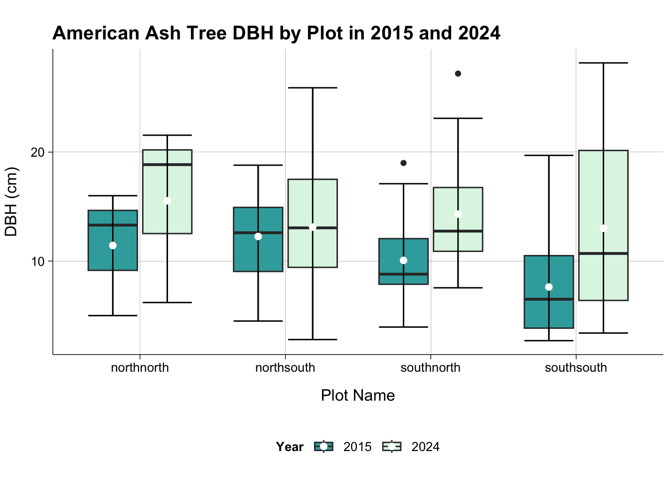
#Statistical Analysis

#T-Test
dat_all_ash <- dat_all |>
  filter(species_name == "American Ash")

t.test(dbh_2024 ~ hl_density, data = dat_all_ash)
    Welch Two Sample t-test

data:  dbh_2024 by hl_density
t = 0.081381, df = 103.96, p-value = 0.9353
alternative hypothesis: true difference in means between group High Density and group Low Density is not equal to 0
95 percent confidence interval:
 -2.382149  2.586035
sample estimates:
mean in group High Density  mean in group Low Density
13.38064 13.27870 t.test(dbh_2015 ~ hl_density, data = dat_all_ash)
    Welch Two Sample t-test

data:  dbh_2015 by hl_density
t = -4.7587, df = 102.88, p-value = 6.384e-06
alternative hypothesis: true difference in means between group High Density and group Low Density is not equal to 0
95 percent confidence interval:
 -5.503890 -2.265709
sample estimates:
mean in group High Density  mean in group Low Density
                  8.320635                  12.205435
#DBH vs plot location ANOVA
model_2015_ash <- aov(dbh_2015 ~ plot_name, data = dat_all_ash)
summary(model_2015_ash) Df Sum Sq Mean Sq F value Pr(>F)
plot_name 3 479.7 159.91 8.888 2.66e-05 ***
Residuals 105 1889.2 17.99
---
Signif. codes: 0 '***' 0.001 '**' 0.01 '*' 0.05 '.' 0.1 ' ' 1model_2015_ash$coefficients (Intercept) plot_namenorthsouth plot_namesouthnorth plot_namesouthsouth
11.433333 0.825969 -1.369444 -3.810000 tukey15 <- TukeyHSD(model_2015_ash)
print(tukey15) Tukey multiple comparisons of means
95% family-wise confidence level
Fit: aov(formula = dbh_2015 ~ plot_name, data = dat_all_ash)
$plot_name
diff lwr upr p adj
northsouth-northnorth 0.825969 -5.786793 7.438731 0.9879593
southnorth-northnorth -1.369444 -8.275206 5.536317 0.9546804
southsouth-northnorth -3.810000 -10.413171 2.793171 0.4373882
southnorth-northsouth -2.195413 -5.304217 0.913390 0.2589815
southsouth-northsouth -4.635969 -6.997533 -2.274405 0.0000081
southsouth-southnorth -2.440556 -5.528906 0.647795 0.1721049plot(tukey15, las = 0 , col = "brown", cex.axis=0.40)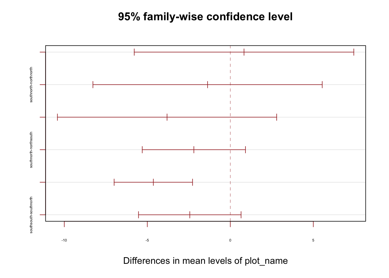
model_2024_ash <- aov(dbh_2024 ~ plot_name, data = dat_all_ash)
summary(model_2024_ash)
Df Sum Sq Mean Sq F value Pr(>F)
plot_name 3 37 12.36 0.28 0.839
Residuals 102 4496 44.08
3 observations deleted due to missingnessmodel_2024_ash$coefficients (Intercept) plot_namenorthsouth plot_namesouthnorth plot_namesouthsouth
15.533333 -2.411938 -1.223039 -2.520233 tukey24 <- TukeyHSD(model_2024_ash)
print(tukey24) Tukey multiple comparisons of means
95% family-wise confidence level
Fit: aov(formula = dbh_2024 ~ plot_name, data = dat_all_ash)
$plot_name
diff lwr upr p adj
northsouth-northnorth -2.4119380 -12.767477 7.943601 0.9292169
southnorth-northnorth -1.2230392 -12.082758 9.636679 0.9910924
southsouth-northnorth -2.5202326 -12.875772 7.835307 0.9202635
southnorth-northsouth 1.1888988 -3.779376 6.157173 0.9238205
southsouth-northsouth -0.1082946 -3.848276 3.631687 0.9998438
southsouth-southnorth -1.2971933 -6.265468 3.671081 0.9037437plot(tukey24, las = 0 , col = "brown", cex.axis=0.40)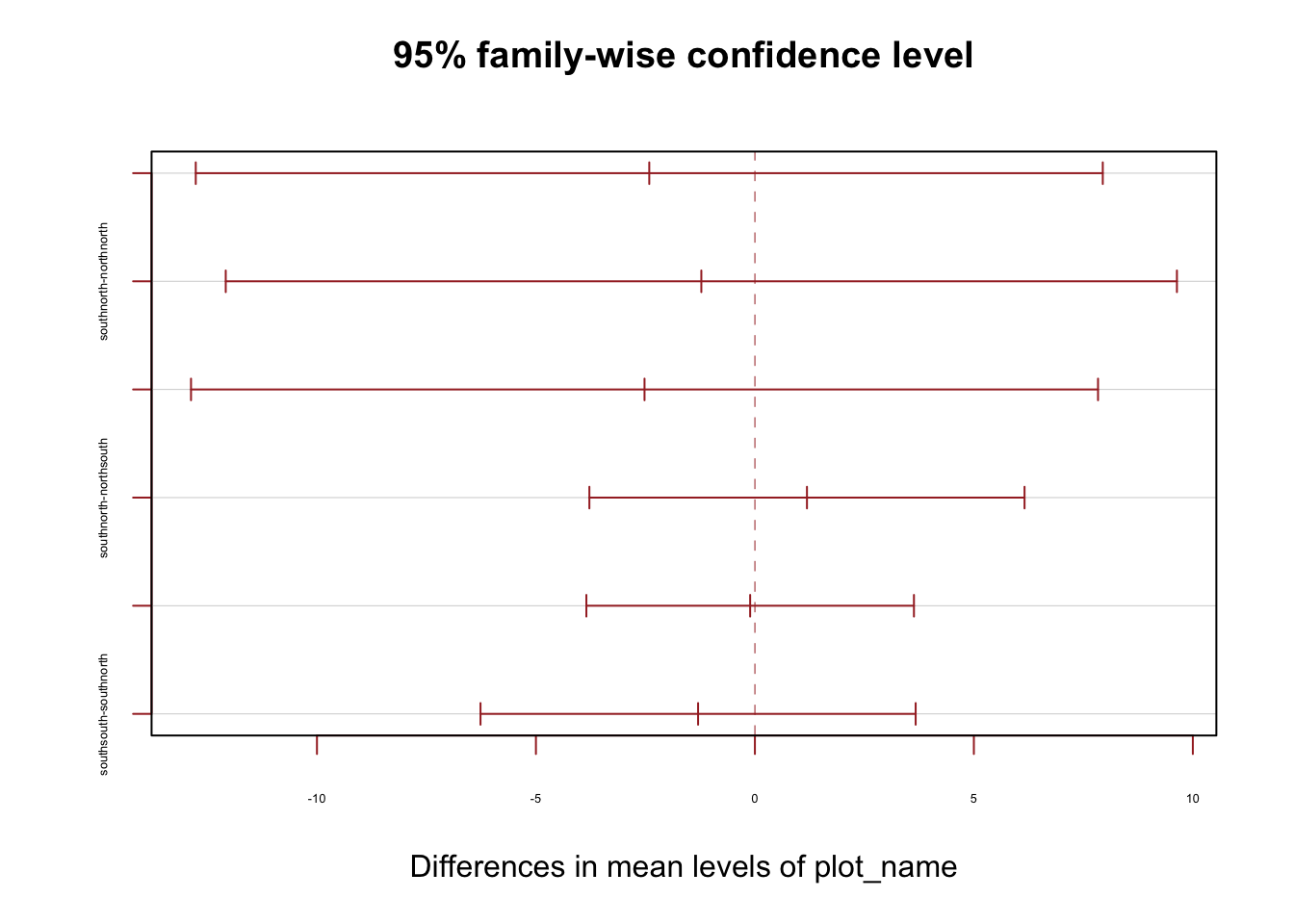
Growth Factor by Plot
dat_all |>
  ggplot(aes(hl_density, growth_factor, fill = hl_density)) +
  geom_boxplot() +
  stat_boxplot(geom = "errorbar",
               width = 0.25) +
  geom_boxplot() +
  theme_publish() +
  scale_fill_manual(values = c("#38AAAB", "#DEF5E5"))+
  theme(panel.grid.major = element_line(colour = "black",
                                        linewidth = 0.05)) +
  labs(title = "Growth Factor by Ash Tree Density",
       x = "Ash Tree Density",
       y = "Growth Factor (cm/yr)",
       fill = "Tree Density")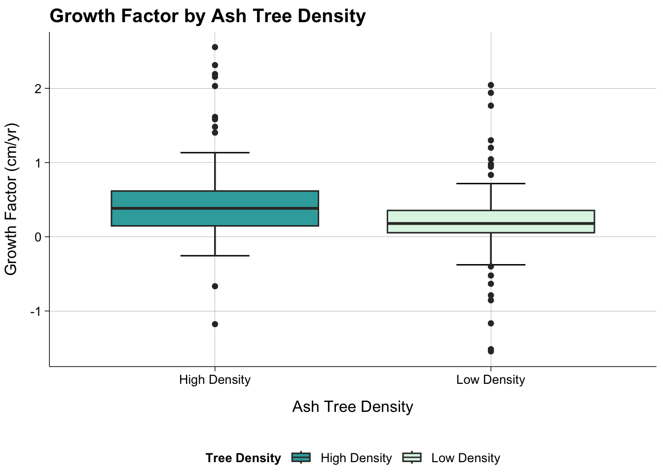
dat_all |>
ggplot(aes(plot_name, growth_factor, fill = plot_name)) +
  stat_boxplot(geom = "errorbar",
               width = 0.25) +
  geom_boxplot() +
  theme_publish() +
  scale_fill_viridis_d(option = "mako") +
  theme(panel.grid.major = element_line(colour = "black",
                                        linewidth = 0.05)) +
  labs(title = "Growth Factor by Plot",
       x = "Plot Name",
       y = "Growth Factor (cm/yr)",
       fill = "Plot Name")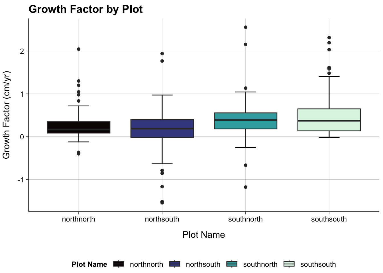
#Statistical Analysis
#T-test
t.test(growth_factor ~ hl_density, data = dat_all)
    Welch Two Sample t-test

data:  growth_factor by hl_density
t = 3.8956, df = 230.52, p-value = 0.0001284
alternative hypothesis: true difference in means between group High Density and group Low Density is not equal to 0
95 percent confidence interval:
 0.1299268 0.3958522
sample estimates:
mean in group High Density  mean in group Low Density
0.4635862 0.2006966 ggqqplot(dat_all, x = "growth_factor", facet.by = "hl_density")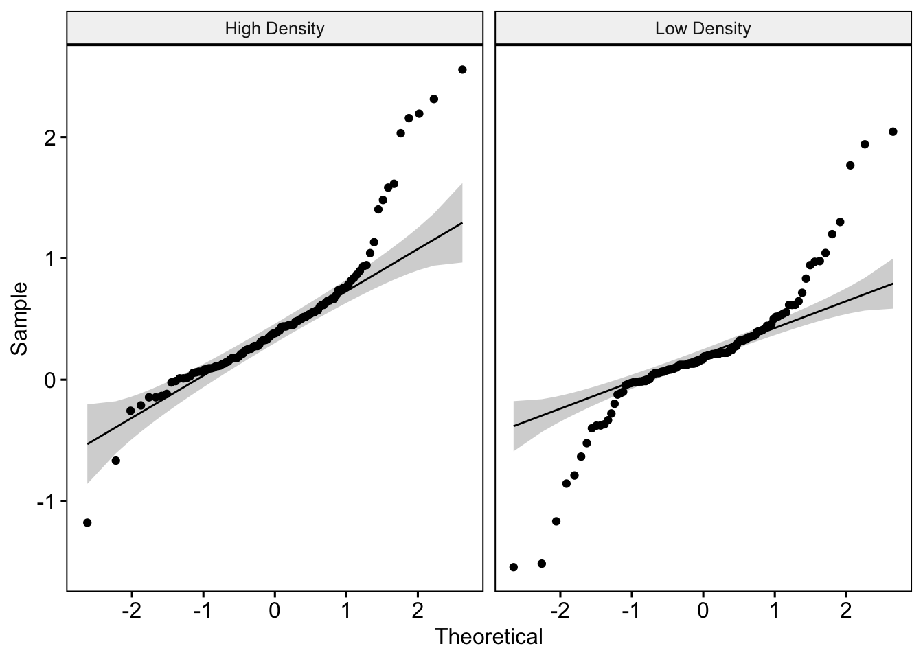
#dat_all <- dat_all |>
#  mutate(log_growth = log(growth_factor + 2))

#ggqqplot(dat_all, x = "log_growth", facet.by = "hl_density")
#t.test(log_growth ~ hl_density, data = dat_all)
#commented out log transform doesn't help

#The true difference in mean growth factor between the high density and low density plots is not equal to zero. We are 95% confident that the true difference in mean growth factor between the high and low density plots is between 0.071 and 0.377 cm/yr. p-value = 0.004385.
Growth Factor by Genus
#Rhamnus not shown because there was only 1 indivdiual in 2015 which died by 2024.
dat_all |>
filter(is.na(species_code) == FALSE & species_genus != "Rhamnus") |>
ggplot(aes(reorder(species_genus, growth_factor, mean), growth_factor, fill = (reorder(species_genus, growth_factor, mean)))) +
  stat_boxplot(geom = "errorbar",
               width = 0.25) +
  geom_boxplot() +
  theme_publish() +
  scale_fill_viridis_d(option = "mako") +
  theme(panel.grid.major = element_line(colour = "black",
                                        linewidth = 0.05)) +
  labs(title = "Growth Factor by Genus",
       x = "Genus",
       y = "Growth Factor (cm/yr)",
       fill = "Genus")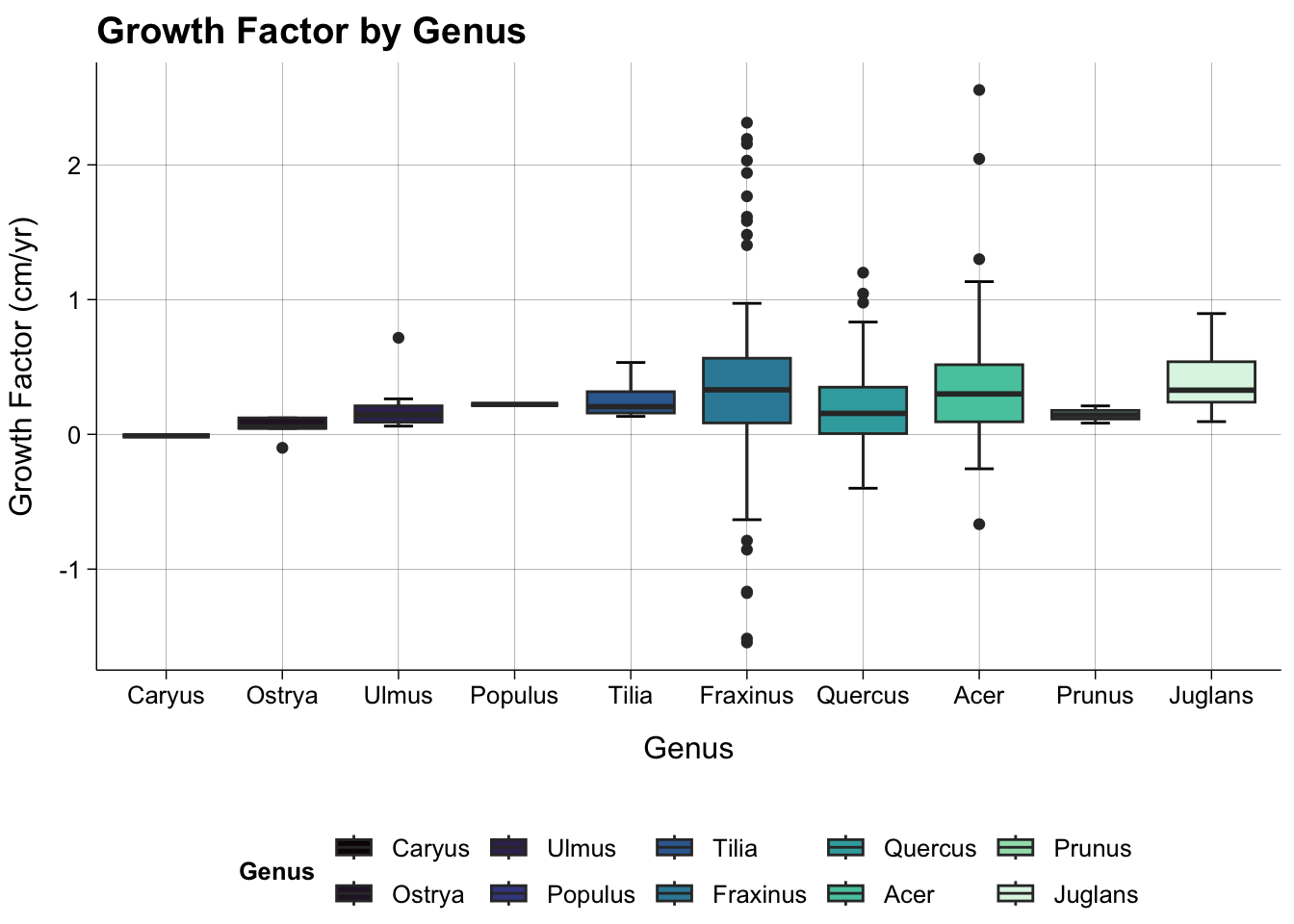
Species and Growth Factor in High and Low Density Plots
#High Density Only
dat_all |>
  group_by(species_name) |>
  summarise(count = n()) |>
  filter(count > 10)
# A tibble: 8 × 2
species_name count
<fct> <int>
1 American Ash 109
2 Bur Oak 25
3 White Oak 19
4 Sugar Maple 15
5 Black Walnut 23
6 Boxelder 11
7 Red Maple 29
8 <NA> 22#There are at least 10 trees of American Ash, Bur Oak, White Oak, Sugar Maple, Black Walnut, Boxelder, Red Maple.
# There are more species (16) in the low density plot vs the high density plot (8)
dat_all |>
group_by(hl_density) |>
summarize(unique_species_n = n_distinct(species_name))# A tibble: 2 × 2
hl_density unique_species_n
<chr> <int>
1 High Density 8
2 Low Density 16dat_all |>
filter(is.na(species_code) == FALSE & hl_density == "High Density") |>
filter(species_name %in% c("American Ash", "Bur Oak", "White Oak", "Sugar Maple", "Black Walnut", "Boxelder", "Red Maple")) |>
ggplot(aes(reorder(species_name, growth_factor, mean), growth_factor, fill = (reorder(species_name, growth_factor, mean)))) +
stat_boxplot(geom = "errorbar",
width = 0.25) +
geom_boxplot() +
theme_publish() +
scale_fill_viridis_d(option = "mako") +
theme(panel.grid.major = element_line(colour = "black",
linewidth = 0.05)) +
labs(title = "Growth Factor by Species in High Ash Density Plots",
x = "Species",
y = "Growth Factor (cm/yr)",
fill = "Species")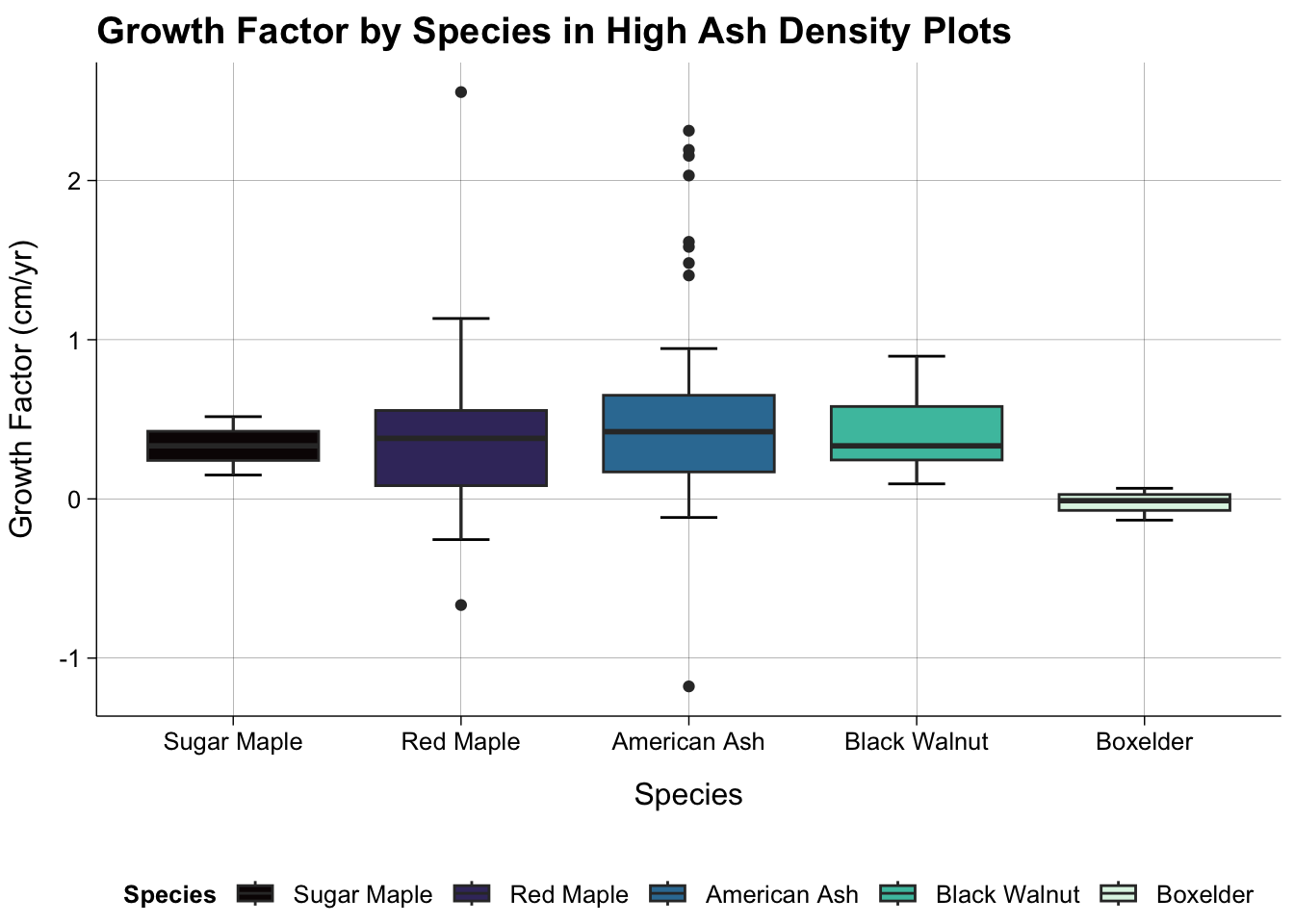
#Low Density Only
dat_all |>
filter(is.na(species_code) == FALSE & hl_density == "Low Density") |>
filter(species_name %in% c("American Ash", "Bur Oak", "White Oak", "Sugar Maple", "Black Walnut", "Boxelder", "Red Maple")) |>
ggplot(aes(reorder(species_name, growth_factor, mean), growth_factor, fill = (reorder(species_name, growth_factor, mean)))) +
  stat_boxplot(geom = "errorbar",
               width = 0.25) +
  geom_boxplot() +
  theme_publish() +
  scale_fill_viridis_d(option = "mako") +
  theme(panel.grid.major = element_line(colour = "black",
                                        linewidth = 0.05)) +
  labs(title = "Growth Factor by Species in Low Ash Density Plots",
       x = "Species",
       y = "Growth Factor (cm/yr)",
       fill = "Species")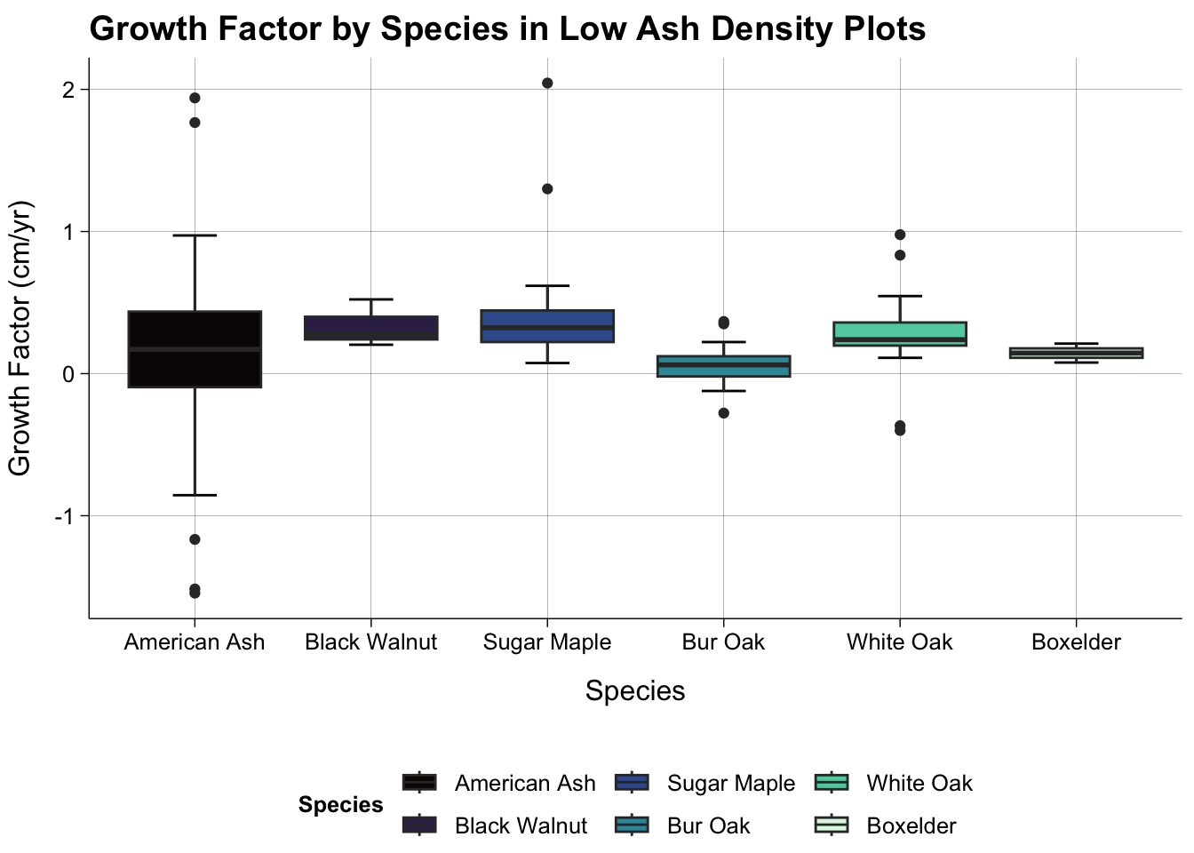
#There aren't any Bur Oak or White Oak in the High Density plots.